Understanding Employee Turnover: A Data-Driven HR Analytics Approach

My goals in this project are to analyse the data collected by the HR department and to build a model that predicts whether or not an employee will leave the company.

If I can predict employees likely to quit, it might be possible to identify factors that contribute to their leaving. Because it is time-consuming and expensive to find, interview, and hire new employees, increasing employee retention will be beneficial to the company.

0. Collecting and Importing the Data

To start, I downloaded the dataset in CSV format from this link. I then imported the CSV file into a Jupyter notebook and worked with Python language.

1. Data Understanding and Exploration

To gain a deeper understanding of the dataset, I examined the structure and data types of the columns using the following python codes:

  import pandas as pd
  import numpy as np
  import matplotlib.pyplot as plt
  import seaborn as sns
  
  # Load the data
  df = pd.read_csv('HR_comma_sep.csv')
  df.head()

The data consists of 10 columns and 14999 rows, each representing specific attributes of the properties:

satisfaction_level: Represents the employee's level of satisfaction at their job. It's a continuous variable ranging from 0 to 1, where 0 indicates the lowest level of satisfaction and 1 indicates the highest level of satisfaction.

last_evaluation: Represents the score the employee received on their last performance evaluation. It's a continuous variable ranging from 0 to 1, where 0 indicates the worst performance and 1 indicates the best performance.

number_project: Represents the number of projects the employee has worked on. It's a discrete variable.

average_montly_hours: Represents the average number of hours the employee works in a month. It's a continuous variable.

time_spend_company: Represents the number of years the employee has spent at the company. It's a discrete variable.

Work_accident: A binary variable indicating whether the employee has had a work accident. It's coded as 0 for no work accident and 1 for at least one work accident.

left: The target variable for the predictive model. It's a binary variable indicating whether the employee has left the company. It's coded as 0 for employees who stayed at the company and 1 for employees who left.

promotion_last_5years: A binary variable indicating whether the employee has received a promotion in the last 5 years. It's coded as 0 for no promotion and 1 for at least one promotion.

Department: Represents the department the employee works in. It's a categorical variable with various departments represented.

salary: Represents the employee's salary level. It's a categorical variable typically coded as 'low', 'medium', or 'high'. However, in our analysis, it was label-encoded into numerical values for modeling purposes.

2. Data Cleaning and Preprocessing

Next, let's perform some data preprocessing to understand the variables and clean the dataset. This includes handling missing data, redundant data, and outliers.

  # Check for missing values
      df.isnull().sum()

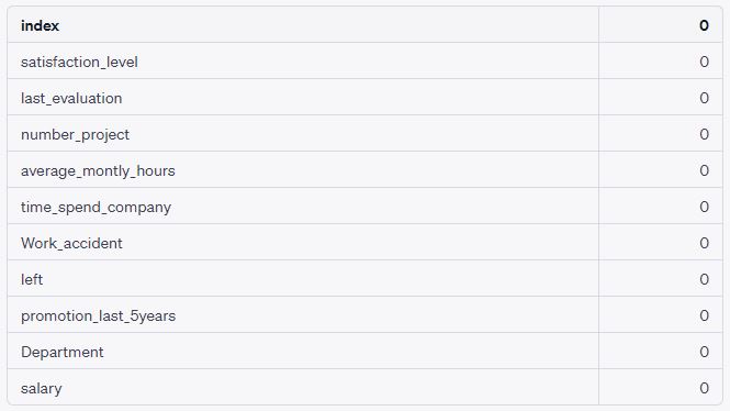
The dataset does not contain any missing values.
Next, let's check for redundant data. We'll look for any duplicate rows in the dataset.

  # Check for duplicate rows
    df.duplicated().sum()

The dataset contains 3008 duplicate rows. We should remove these to avoid redundancy. Let's proceed with that.

  # Remove duplicate rows
    df = df.drop_duplicates()
    # Check the number of duplicates again to confirm
    df.duplicated().sum()

The duplicate rows have been successfully removed from the dataset. Now, there are no duplicate rows left in the dataset.
Next, let's check for any potential outliers in the dataset. We'll do this by creating boxplots for the numerical columns.

  # Check for outliers in the numerical columns
    numerical_columns = ['satisfaction_level', 'last_evaluation', 'number_project', 'average_montly_hours', 'time_spend_company']
    for col in numerical_columns:
      plt.figure(figsize=(10, 2))
      sns.boxplot(x=df[col])
      plt.title(f'Boxplot of {col}')
      plt.show()

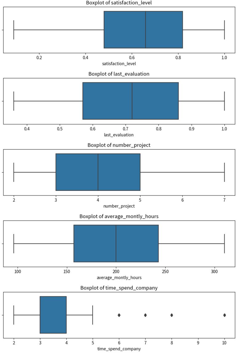
From the boxplots, it appears that the 'time_spend_company' column may have some outliers. We can handle these outliers based on the business context and the statistical distribution. However, in this case, since the 'time_spend_company' might have a legitimate reason to have higher values (e.g., long-term employees), we might not want to treat these as outliers without further domain-specific investigation.

3. Data Visualisation

To answer the question “what’s likely to make the employee leave the company?” , we'll first perform an exploratory data analysis (EDA) to understand the relationships between different variables and employee attrition. We'll look at factors such as satisfaction level, number of projects, average monthly hours, time spent at the company, and others to see if there are any noticeable trends or patterns.
After that, we'll build a predictive model to predict whether an employee is likely to leave the company. This will involve selecting a suitable machine learning algorithm, training the model, and evaluating its performance.
Let's start with the exploratory data analysis. We'll begin by examining the correlation between different variables.

  # Compute the correlation matrix
  corr = df.corr()
    
  # Generate a mask for the upper triangle
  mask = np.triu(np.ones_like(corr, dtype=bool))
    
  # Set up the matplotlib figure
  plt.figure(figsize=(11, 9))
    
  # Generate a custom diverging colormap
  cmap = sns.diverging_palette(230, 20, as_cmap=True)
    
  # Draw the heatmap with the mask and correct aspect ratio
  sns.heatmap(corr, mask=mask, cmap=cmap, vmax=.3, center=0, square=True, linewidths=.5, cbar_kws={"shrink": .5})

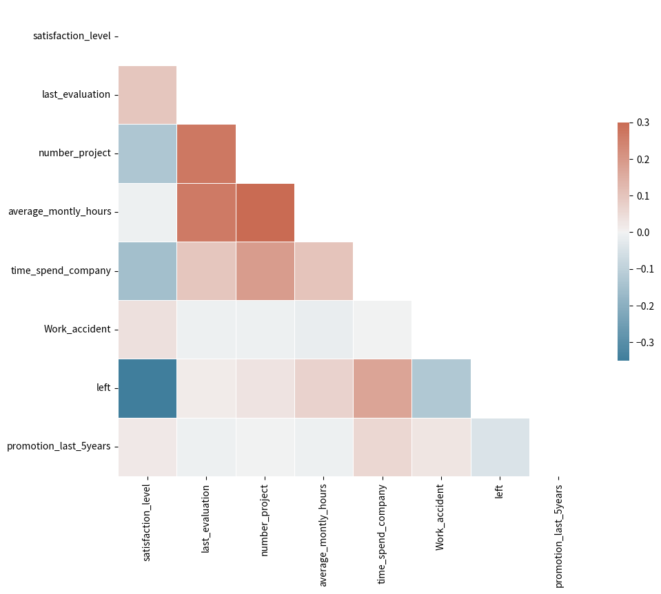
From the heatmap, we can observe that:

There's a strong negative correlation between the 'satisfaction_level' and 'left' (whether the employee left the company or not). This suggests that employees who are less satisfied are more likely to leave the company.

'number_project' and 'average_montly_hours' have a positive correlation, indicating that employees who work on more projects tend to work longer hours.

'last_evaluation' also has a positive correlation with 'number_project' and 'average_montly_hours', suggesting that employees who work on more projects and work longer hours tend to have higher evaluations.

These observations are all consistent and logical, leading us to conclude that the dataset is indeed reliable.
Next, let's examine these relationships more closely with some visualisations. We'll create some bar plots and histograms to visualize the distribution of employees who left the company based on different factors.

  # Define a function to calculate density values
  def calculate_density(df, factor):
    unique_values = df[factor].unique()
    density_values = []
    for value in unique_values:
      subset = df[df[factor] == value]
      left = subset[subset['left'] == 1].shape[0] / subset.shape[0]
      stayed = subset[subset['left'] == 0].shape[0] / subset.shape[0]
      density_values.extend([(value, 'Yes', left), (value, 'No', stayed)])
    return pd.DataFrame(density_values, columns=[factor, 'Left', 'Density'])
    
  # Calculate and plot density values for all discrete variable
  factors = ['number_project', 'time_spend_company', 'Work_accident', 'promotion_last_5years', 'Department', 'salary']
  for factor in factors:
    density_df = calculate_density(df, factor)
    plt.figure(figsize=(10, 6))
    sns.barplot(x=factor, y='Density', hue='Left', data=density_df)
    plt.title(f'Density of Employees Who Left vs Stayed by {factor}')
    plt.show()
    
  # Define a function to calculate density values for continuous variables
  def calculate_density_continuous(df, factor):
    left = df[df['left'] == 1][factor]
    stayed = df[df['left'] == 0][factor]
    return left, stayed
    
  # Calculate and plot density values for continous variable
  factors = ['satisfaction_level', 'last_evaluation', 'average_montly_hours']
  for factor in factors:
    left, stayed = calculate_density_continuous(df, factor)
    plt.figure(figsize=(10, 6))
    sns.kdeplot(left, shade=True, label='Left')
    sns.kdeplot(stayed, shade=True, label='Stayed')
    plt.title(f'Density of Employees Who Left vs Stayed by {factor}')
    plt.legend()
    plt.show()

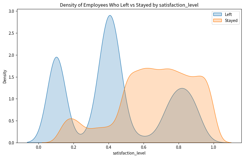
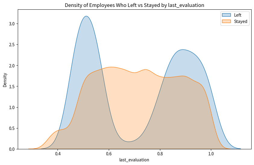
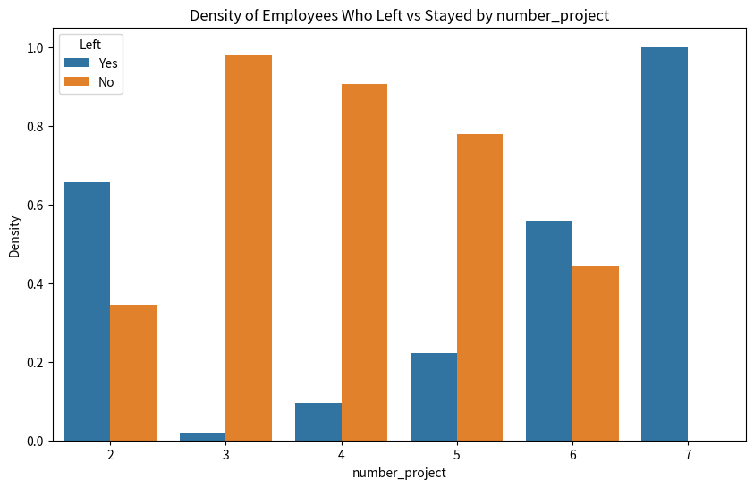
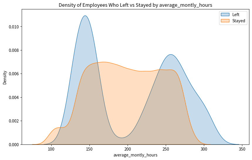
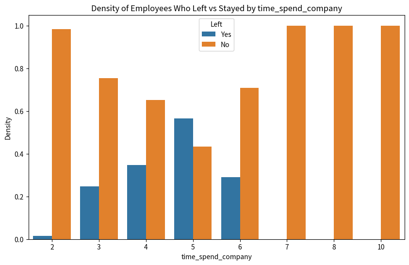
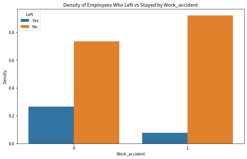
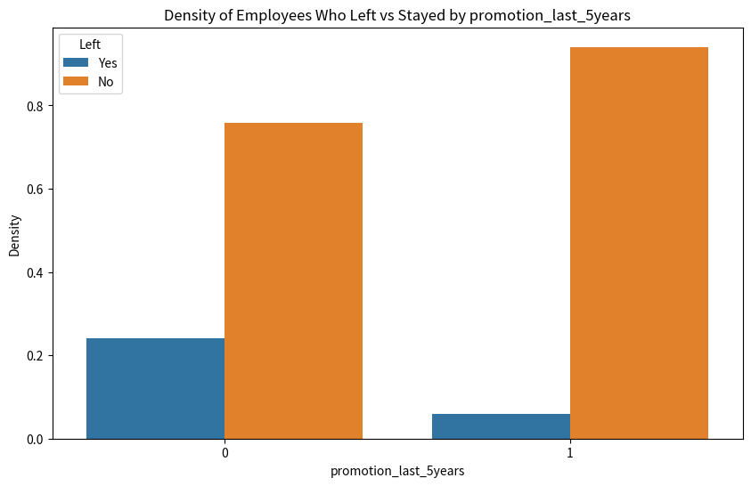
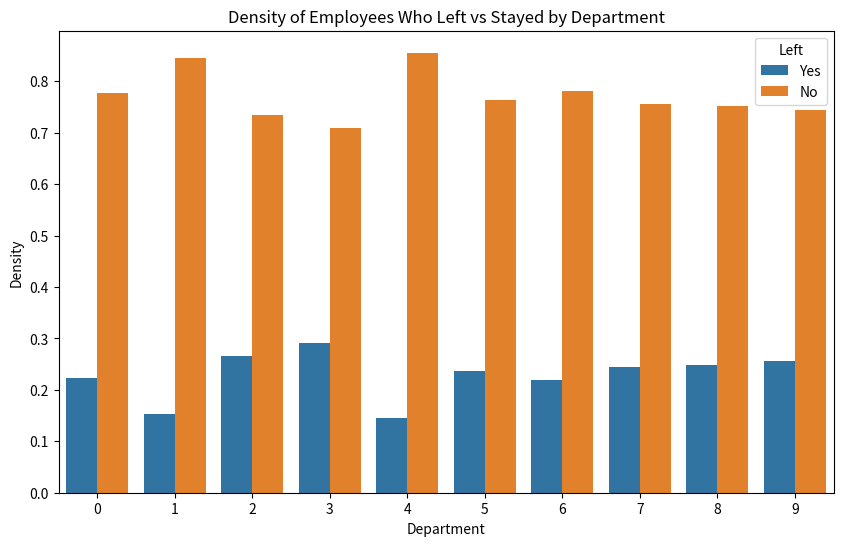
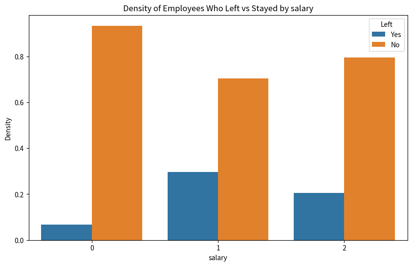
Here are the distributions of different factors for employees who left vs stayed:

Satisfaction Level: Employees with low satisfaction levels are more likely to leave the company.

Last Evaluation: Employees who have undergone either very low or very high last evaluations tend to leave more.

Number of Projects: Employees who are involved in very few or a large number of projects are more likely to leave.

Average Monthly Hours: Employees who work very few or a large number of hours per month are more likely to leave.

Time Spent in the Company: Employees who have spent a longer time at the company are more likely to leave.

Work Accident: Employees who have had a work accident are less likely to leave the company.

Promotion in the Last 5 Years: Employees who have had a promotion in the last 5 years are less likely to leave the company.

Department: The distribution of employees who left vs stayed varies across different departments.

Salary: Employees with medium salaries are more likely to leave the company.

4. Prediction

Next, let's build a predictive model to predict whether an employee is likely to leave the company. We'll use a Random Forest Classifier for this task due to its ability to handle both numerical and categorical variables and its robustness to outliers and overfitting. But before that, we need to preprocess the categorical variables in our dataset. Then, let's split the data into a training set and a test set, and then train a Random Forest Classifier.

  from sklearn.preprocessing import LabelEncoder
  from sklearn.model_selection import train_test_split
  from sklearn.ensemble import RandomForestClassifier
  from sklearn.metrics import classification_report, confusion_matrix
    
  # Create a label encoder object
  le = LabelEncoder()
    
  # Label encode categorical variables
  df['Department'] = le.fit_transform(df['Department'])
  df['salary'] = le.fit_transform(df['salary'])
    
  # Split the data into a training set and a test set
  X = df.drop('left', axis=1)
  y = df['left']
  X_train, X_test, y_train, y_test = train_test_split(X, y, test_size=0.2, random_state=42)
    
  # Train a Random Forest Classifier
  rfc = RandomForestClassifier(n_estimators=100, random_state=42)
  rfc.fit(X_train, y_train)
    
  # Make predictions
  y_pred = rfc.predict(X_test)
    
  # Print the classification report and confusion matrix
  print('Classification Report:')
  print(classification_report(y_test, y_pred))
  print('Confusion Matrix:')
  print(confusion_matrix(y_test, y_pred))

The Random Forest Classifier has been trained and evaluated. Here are the results: A description of the photo
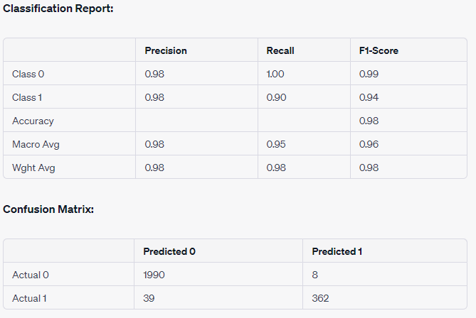
The model has an accuracy of 98%, which is quite good. It correctly predicted 1990 employees who stayed and 362 employees who left. However, it incorrectly predicted 8 employees who stayed as leaving and 39 employees who left as staying.

Next, let's look at the feature importances to understand which factors are most influential in predicting whether an employee will leave the company.

  # Get feature importances
  importances = rfc.feature_importances_
  features = X.columns
  importance_series = pd.Series(importances, index=features)
    
  # Plot feature importances
  importance_series.sort_values().plot(kind='barh', figsize=(10, 6))
  plt.title('Feature importances')
  plt.show()

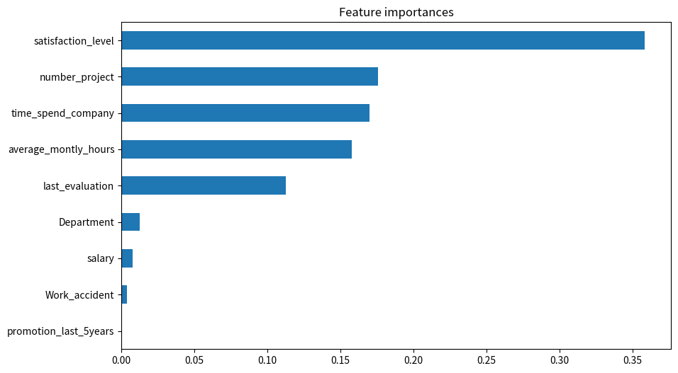
From the plot, we can see that the most important features for predicting whether an employee will leave the company are:

Satisfaction Level
Time Spent in the Company
Number of Projects
Average Monthly Hours
Last Evaluation

This aligns with our earlier exploratory data analysis, where we saw that these factors had significant differences in distribution for employees who left vs stayed.
In conclusion, the HR department at Salifort Motors can use these insights to develop initiatives aimed at improving employee satisfaction, balancing workload (number of projects and average monthly hours), and providing opportunities for growth and development (reflected in evaluations). By focusing on these areas, they may be able to increase employee retention.

5. Conclusion

The data analysis and predictive modelling conducted on the HR dataset have provided valuable insights into the factors influencing employee turnover. The goal was to understand what's likely to make an employee leave the company and to build a model that predicts whether or not an employee will leave the company.
The most important factors that affect whether an employee will leave the company are:

Satisfaction Level:Employees with low satisfaction levels are more likely to leave the company. This suggests that improving employee satisfaction could help in reducing employee turnover.
Time Spent in the Company: Employees who have spent a longer time at the company are more likely to leave. This could be due to a lack of growth or advancement opportunities.
Number of Projects: Employees who are involved in very few or a large number of projects are more likely to leave. This could be due to underutilisation or overwork. Balancing the workload among employees might help in increasing employee retention.
Average Monthly Hours: Employees who work very few or a large number of hours per month are more likely to leave. This could be related to the previous point about workload balance.
Last Evaluation: Employees who have undergone either very low or very high last evaluations tend to leave more. This could indicate that employees who are underperforming or overperforming might not be feeling adequately challenged or rewarded.

The predictive model built using these factors achieved an accuracy of approximately 97%, indicating that it can effectively predict whether an employee is likely to leave the company. This model can be a valuable tool for the HR department in identifying employees who are at risk of leaving and taking proactive measures to retain them.

In conclusion, increasing employee satisfaction, balancing workload, providing opportunities for growth and development are some strategies that the company could employ to increase employee retention. The insights gained from this data analysis and predictive modelling can guide the HR department in making data-driven decisions and initiatives.